Pharmacophore an International Research Journal
Statistical Approaches for Dissolution Profile Comparisons of Metformin Film-Coated Tablets
Ivana Mitrevska1*, Ljupco Pejov2,3, Stefan Trajkovikj1, Katerina Brezovska4, Aneta Dimitrovska4, Sonja Ugarkovic1
|
|
|
ABSTRACT
The objective of this work was to apply several statistical approaches to profile comparison on dissolution data of Metformin immediate release film-coated tablets to assure that the developed formulation of the test product that is similar to the reference product (Glucophage film-coated tablets). The evaluated medicinal product belongs to BCS Class III (high solubility, low permeability). The similarity testing of the dissolution profile was performed on the highest strength of the dosage form, following the regulatory requirements for bioequivalence study. The obtained results showed that the simple standard difference and similarity (f1 and f2)-factors are not applicable and therefore practically not useful for comparison of dissolution profiles because one of the regulatory requirements that the relative standard deviation or coefficient of variation of any product should be less than 20% for the first point and less than 10% from second to last time point, which was not achieved in the present case. Therefore, more advanced multivariate methods such as model-dependent approaches coupled to multivariate statistics, the multivariate model-independent approach based on generalized statistical distance (such as e.g. Mahalanobis distance) have been applied for evaluation of dissolution profiles. This approach appeared to provide extra arguments when deciding if two profiles are similar, as it allows for a better description of the dissolution processes (in the sense of e.g. the rate and amount of the active substance dissolved) and thus a better prediction of in vivo performance. Comparison with traditional methods such as those based on fit-factors is made, and their shortcomings pinpointed out. Dissolution profiles can be tested for differences in both level and shape by multivariate-based methods and these methods provide detailed information about dissolution data, which can be useful also in formulation development to achieve the final goal – match the actual performance of the released test product to the performance of a target reference product.
Keywords: Metformin film-coated tablets; comparison of dissolution profiles; multivariate statistic; model-dependent method; model-independent method.
Introduction
Whenever a new solid dosage form is developed or produced, it is necessary to ensure that drug dissolution occurs appropriately. Several studies documented that a combination of herbal products with a synthetic drug is useful compared to single treatment as observed in various pathological situations [1]. Despite the significant range of ready-made medicines, the preparation of extemporaneous medicines according to individual prescriptions does not lose its relevance today [2]. Complementary and alternative medicine refers to diverse medical and health care systems, products, and practices, which are not part of the usual medications and treatments [3]. Combining bioactive nanomaterials with a biomaterial scaffold indicates a successful development of a localized long-term treatment [4]. Dissolution tests are used to guide the development of new formulations, monitor the quality of drug products, assess the potential impact of post-approval changes on product performance, and, in some cases, predict the in vivo performance of the drug product. In vitro dissolution as an important element in drug development, under certain conditions can be used as a surrogate for the assessment of bioequivalence (BE). Expensive in vivo bioequivalence testing can be waived if If dissolution profile similarity is demonstrated between different strengths of the medicinal product. Also, several biowaivers and post-approval changes may be obtained for regulatory purposes if similarities in dissolution are demonstrated between different dosage strengths or between the test and reference drug products [5].
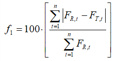
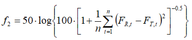
To this aim, the f2 method proposed by Moore and Flanner [6] is, due to its simplicity, the metric of choice by both the EMA and the FDA. With this metric (often referred to as a similarity factor), if two dissolution profiles are equal, a value of 100 is obtained. An average difference of 10% at all measured sampling time points results in an f2 value of 50, which has been considered as the cut-off threshold to conclude the similarity between two dissolution profiles. Similarly, the f1 (or difference factor) metric has been defined analogously, keeping the simplicity in both the definition and physical meaning of the computed parameter [6, 7]. The main advantages of the f1 and f2 metrics lie in the fact that they are easy and straightforward to compute and, at the same time, they provide a single number to describe the comparison of dissolution profile data (consisting of measured solubility at different time points). In a sense, most simplistically, these two parameters aim to map and quantify the similarity of two-time series by a single numerical parameter. However, there are disadvantages. The f1 and f2 factors do not take into account the variability or correlation structure in the data, the level of confidence associated with this method is uncertain, and its statistical power is rather low. Since the definition equations for f1 and f2 have not arisen from a rigorous statistical-based theoretical approach (i.e. are in a sense non-statistical methods for the comparison of dissolution profile data), but rather from a purely intuitive viewpoint, it is essentially not possible to know the probability of concluding that the test and reference mean profiles are the same, when they are different. Therefore, to avoid the overall risk of incorrectly concluding that the mean dissolution profiles are different, obviously, a more advanced approach (such as e.g. the multivariate approach based on Mahalanobis distance), which takes the variability and correlation structure into account in measuring the difference between mean dissolution profiles, should be carried out. Following the FDA guidance, after the estimation of the Mahalanobis distance between its profiles, the corresponding 90% one-sided confidence interval of true MSD, and comparison of the upper limit with the similarity pre-established limit, the evaluation of the similarity between test and reference samples is done [7]. Under this protocol, the test batch is considered to be similar to the reference batch if the upper limit of the confidence interval is not larger than (i.e. does not exceed) the similarity limit.
Such a multivariate approach may be used in conjunction with a method for data assessment which could be either model-independent or model-dependent. The characterization of the data assessment method as model-dependent or model-independent depends on the values which are used to perform the calculation. A model-independent method uses the dissolution data in their native (“raw”) form. The model-dependent methods, however, are based on different model functions, which are used to describe the dissolution profile, often based on fitting the experimental data by a least-squares routine. Once a suitable function has been selected, the dissolution profiles are evaluated not by assessing the original (as-measured, i.e. “raw” data), but rather the parameters of the model functions obtained by least-squares fitting to the experimental data.
The present study addresses different variants of multivariate statistical procedures as an alternative methodology for evaluation of the similarity of two in vitro dissolution profiles, in comparison to the similarity factor f2 as a criterion for similarity assessment, as proposed in the EMA and SUPAC-IR guidelines. It is demonstrated that the variety of tested methods allow similar conclusions to be drawn similarly to the time-series representing the dissolution curves (albeit not for all of the studied cases). However, the model-dependent approaches, fit-factors, and ratio tests appear to be less informative than the correlation approach.
Experimental procedure
Equipment and Materials
Two batches of reference drug products (Glucophage 1000 mg film-coated tablets) were purchased at the EU market and test products (Metformin 1000, 850, and 500 mg film-coated tablets) were manufactured by Alkaloid AD Skopje. The following reference drug products were tested: reference, batch no. M2483 (Slovenia), R1; reference, batch no. 16805 (Germany). All other chemicals and reagents were analytical grades.
In vitro dissolution studies
Testing is carried out at 37 ± 0.5°C and 75 rpm using calibrated Apparatus II (paddle) with 1000 mL ± 1% of each medium. Sampling for all dissolution tests is performed at 5, 10, 15, 20, 30, and 45 minutes. In all cases, media are deaerated and filtered through a 0.45 μm regenerated cellulose membrane filter. The samples are taken manually through a 10 mL syringe, connected to a stainless steel sampling cannula. At each sampling time, 10 ml of the medium is removed and filtered through a 0.20 μm regenerated cellulose membrane filter. Trials are performed with twelve tablets and the obtained values are used for data analysis. Acceptance criteria for not less than 75% (Q) of the labeled content for 45 minutes were established. Samples obtained from dissolution experiments are quantitatively analyzed using a UV-VIS spectrophotometric method previously validated.
Preliminary analyses concerning the similarity of the dissolution profiles
A preliminary analysis of dissolution data was carried out by plotting of “mean dissolution profiles” ( ; test vs. reference sample) with error bars extending to ±σ, as well as with 95 % confidence intervals. An overlap between 95 % confidence intervals evidenced at each time point was considered as a strong indication of the similarity between the investigated time series (though, of course, not definite or quantitative). We have proceeded with our analysis implementing approaches that fall within two main categories which have been proposed in the literature for this purpose: (i) model-independent and (ii) model-dependent ones [7].
We have computed difference and similarity factors (f1 and f2 respectively), by the standard formulas [5-7]:
 (1)
(1)
 (2)
(2)
In (1) and (2), FR,t, and FT,t denote the percentages of dissolved reference and test samples, respectively.
These two quantities were computed considering both the “mean dissolution profiles” of the test and reference batches – i.e. as “mean test” vs. “mean reference” (as is usually recommended in the regulative [8, 9]) as well as for each of the 12 test samples against the “mean reference” [10, 11]. In the latter case, also the standard error was computed to get a better insight into the data variability. However, note that in the case of presently analyzed data sets, two prerequisites that are essential for the similarity factor f2 to be used as a valid indicator of similarity between the compared sets are not fulfilled. Namely, in the case of the test product, considering solubility at pH 6.8, more than one mean value of F is larger than 85 % (the last two ones, actually). At the same time, the relative standard deviation (coefficient of variation) is larger than 10 % at several time points in the case of reference products at all pH values at which studies have been performed, and this also appeared to be the case with the test product as well at pH 6.8. The computed f2 values are, therefore, in this context presented just for comparison purposes, and not to derive definitive conclusions concerning the similarity of dissolution profiles. Due to the known deficiencies in the reliability of the computed values of f2 and the sensitivity of this parameter on the number of experimental time points that have been used for computation, we have made numerous computations by slightly different routes, i.e. extending the range of experimental data that are employed for actual computation of f2 (e.g. up to the time point at which solubility > 85 % in the test sample is achieved, or up to the time point at which solubility > 85 % in both test and reference samples is achieved, etc.). The derived conclusions, however, remained unaltered regardless of the particular method implemented for computation.
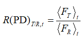
Of the other model-independent methodologies, we have also applied the Ratio test approaches [7, 12]. In the course of the present study, we have implemented the ratio tests of the percent of dissolved test/ratio samples (PD), an area under the concentration curve (AUC) as well as the average dissolution time (ADT). These ratios were calculated between the test and ratio average values at each time point; for example, in the case of PD:
 (3)
(3)
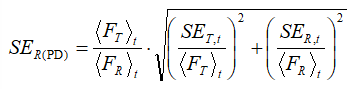
Further, the standard errors (SE) were estimated by the formula:
 (4)
(4)
(SET,t, and SER,t being the standard errors of the test and reference samples at the point t, respectively) and the 90 % confidence intervals (CIs) were calculated as:
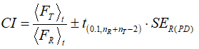 (5)
(5)
In the previous equation, nT and nR denote the number of data in the cases of test and reference samples correspondingly, while  is the value of t-variable with nR +nT –2 degrees of freedom and a confidence limit of 90 %. Analogous procedures were adopted in the case of AUC and ADT ratios. Note that these three procedures are particularly useful in cases when most of the drug has been dissolved in a relatively short time.
In the case of relatively large intra-batch (within-batch) variability, instead of relying on parameters computed based on “pairwise” approaches, multivariate statistical methods are usually recommended to judge the similarity between dissolution profiles of test and reference batches. In the present case, we have therefore implemented a multivariate confidence region procedure, based on 90 % confidence intervals of the generalized statistical distance between the variables. Adopting a multivariate approach, we have explicitly taken into account both the variability and the correlation structure of the compared sets of data, which has certain well-documented advantages over the more conventional (and easier to apply) univariate procedures. In particular, we have based our approach on the Mahalanobis distance DM as a generalized multivariate statistical distance measure [13-17]. Consider a test and a reference product, for which we have carried out a series of p measurements (12 in the present case) for n time points (6 in the present case, excluding t = 0). Each of the 12 measurements at 6-time points in the case of test and reference products thus constitutes a particular realization of a stochastic 1´6 vector x in Â6. We further define a p´n (12´6 in our case) matrix M containing each particular realization of the vector x. The elements of matrix M are further denoted as xi,j, where i = 1,…12, while j = 1,….6. We further denote the vector x and the data matrix M composed by measurements of the reference and test samples by xR(T) and MR(T) respectively.
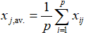
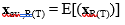
After collecting the matrices MR(T) and vectors xR(T), we have computed the variance-covariance matrices of the reference and test samples, as well as the mean(average)-vectors xav., R(T). The later quantities are defined with the following elements:
 (6)
(6)
i.e.:
 (7)
(7)
where E denotes the mathematical expectation.
The variance-covariance matrices  are, on the other hand, defined with [18]:
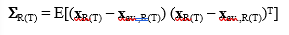 (8)
(8)
where T denotes transposition of the difference vectors (or “centered” x-vectors). Subsequently, we have computed the “pooled” (across the reference and test batches) variance-covariance matrix, defined as:
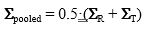 (9)
(9)
As already mentioned before, as a generalized multivariate statistical distance measure [13-17], we have used the Mahalanobis distance DM. We have computed the last quantity as:
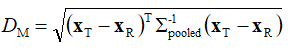 (10)
(10)
where  is the inverse of the pooled variance-covariance matrix. To define the limiting DM value – DM,lim. (“the similarity limit”, in the usual parlance), we have defined a 1´6 vector xlim., the elements of which are the predefined limits expressed as maxima of the tolerable average distances at all time points. With an aid of this vector, DM,lim. is defined as:
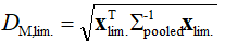 (11)
(11)
Assuming that the data follow the multivariate normal distribution, we have subsequently calculated the 90 % confidence region for the “true” difference between the population-based mean vectors μT – μR from the condition:
 (12)
(12)
In the previous equation, K is a scaling factor, defined with:
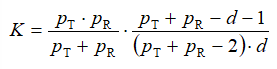 (13)
(13)
where pT and pR are the number of measurements (realizations of the vector components) in the case of test and reference samples respectively (both of which are 12 in the present case), while d is the dimension of the vectors xR(T) (d = 6 in the present case).  , on the other hand, is the 90th percentile of the F-distribution with d and pT + pR – d – 1 degree of freedom. Multiplication by the scaling factor K in (12) is required to obtain a new statistics which is directly comparable to a standard F-distribution. We denote the confidence region calculated from the condition (12) by:
 (14)
(14)
where “L” and “H” imply the “lower” and “higher” limit of the interval. We have derived the conclusion about the similarity of the vectors xR and xT if the condition:
 (15)
(15)
is fulfilled, i.e. if the higher limit of the interval defined with (14) is less then or equal to the limiting value of the Mahalanobis distance.
Upon collection or computation of the data, the phases that follow up in the course of the actual multivariate similarity test are:
 to the Hotelling T2 statistics by the scaling factor K, to enable direct comparison to the standard F-distribution;
We have adopted the following model-dependent approach (procedure) for the present study. First, we have carried out non-linear least-squares fits of the reference samples data with series of widely used model functions, including various variants of the Weibull model functions (with a various number of parameters), Logistic functions (also with a various number of parameters), exponential model function (i.e. time function for the product in a first-order kinetics process), Higuchi model function, quadratic, Hixson-Crowell, Korsmeyer-Peppas, Probit, etc [19, 20]. In this way, we have covered the most widely used functions which are both kinetically- and mechanistically-based. The goodness-of-fit was judged by the values of R2, adjusted R2, and Akaike information criterion (AIC). The best fit has been obtained by the two-parameter Weibull model function of the form:
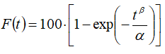 (16)
(16)
Subsequently, the model parameters α and β have been obtained for all available series of data (for both test and reference samples) by non-linear least-squares fitting procedure. After the parameter data had been collected, we have carried out a multivariate similarity test of the model parameters between reference and test batches [13-17], using a procedure that is quite analogous to that implemented in the previous chapter (I. 1. 3).
In this case, out of the original solubility data in the case of the test and reference products, we have derived the set of α and β parameters for each set of measurements (each F = f (t) curve). In a sense, we have mapped the “original” solubility data collected by a series of p measurements (12 in the present case) for n time points (6 in the present case, excluding t = 0) into a set of 12 data vectors containing the mentioned fitting parameters. In other words, this time each of the 12 measurements at 6-time points in test and reference products constitutes a particular realization of a stochastic 1´2 vector x in Â2. We further here construct a 12´2 data matrix M containing each particular realization of the vector x. The elements of matrix M are further denoted as xi,j, where i = 1,…12, while j = 1,2. The vector x and the data matrix M composed by measurements of the reference and test samples are denoted again by xR(T) and MR(T) respectively. The mean (average) – vectors and the covariance matrices are further computed in a manner analogous to that described by the equations (6) – (8) and the pooled covariance matrix is computed by (9) and the Mahalanobis distance by (10). The limiting value – DM,lim. (“the similarity limit”) is in this case computed by defining a 1´2 vector xlim., the elements of which are the empirically defined limits of each of the fitting parameters expressed as maxima of the tolerable average distances of the studied parameters. Again, it is assumed that the data follow the multivariate normal distribution, and the 90 % confidence region for the “true” difference between the population-based mean vectors μT – μR is subsequently calculated from the condition (12). The conclusion concerning the similarity of the vectors xR and xT is at the end derived by checking if the condition (15) is fulfilled, where has been defined by the confidence region (14).
For the present study, we have carried out the multivariate statistical analysis using both the as-obtained (i.e. non-transformed) data for the fitting parameters, as well as the natural logarithm (ln) transformed data. This was done to clarify the possible ambiguity in the assumption for the multivariate normal distribution of the model parameters, which has been discussed to some extent in the literature [13, 14]. However, in our presently studied case, we have obtained conclusive results both with transformed and non-transformed model parameters.
Statistical analyses were carried out in parallel (due to cross-checking of the results) with Wolfram Mathematica 10 [20] and Microsoft Excel 2007 [21]. Note that these program packages are worldwide standards for statistical and mathematical modeling of engineering and scientific data, and have been validated to be used in currently conducted analyses in a wide variety of contexts.
Results and Discussion
Due to several drawbacks of the f2 metric, some conditions were imposed aiming at a convenient characterization of the similarity between dissolution profiles [8]. These are slightly different between the different regulatory agencies, but according to the EMA bioequivalence guideline, the requisites for using the f2 approach are the following: (1) a minimum of three dissolution time points (zero excluded); (2) the dissolution time points should be the same for the two formulations; (3) twelve individual values for every time point for each formulation; (4) not more than one mean value of more than 85% dissolved for any of the formulations and (5) the coefficient of variation (CV) for the 12 units of any of the products being compared should be not more than 20% at the first sampling point and 10% at the remaining sampling time points. These conditions limit the utilization of the f2 metric in several cases, namely in strength biowaivers. In these cases, EMA guideline is requiring in vitro dissolution tests at three different buffers (usually pH 1.2, 4.5 and 6.8) besides the media intended for drug product release, resulting in that frequently dissolution is studied in more demanding conditions and variability in the dissolution profiles becomes more evident. To circumvent this problem, the EMA guideline allows the use of other model-dependent or model-independent methods [6] for dissolution profiles comparison. In this respect, several methods have been proposed [9] but the determination of the similarity limits in terms of multivariate statistical distance (MSD) has been considered by the FDA in the past as a more suitable approach for dissolution profile comparison [7].
As outlined in detail before in the manuscript, two general approaches for comparison of in vitro dissolution profiles of Metformin film-coated tablets and reference (Glucophage film-coated tablets) medicinal products are used: model-dependent and model-independent.
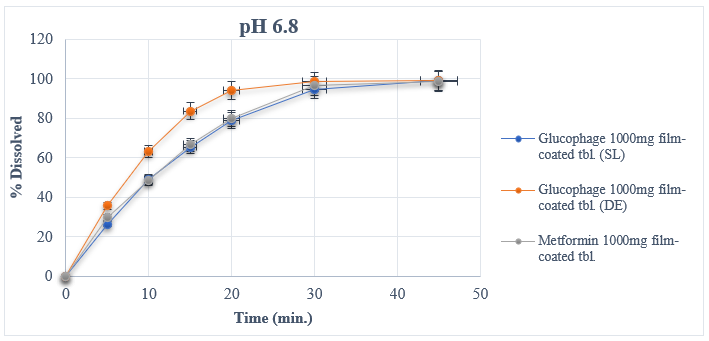
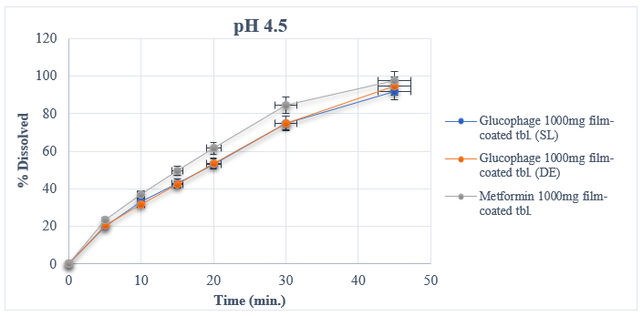
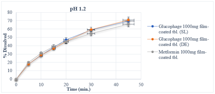
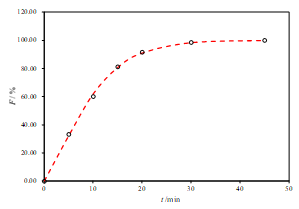
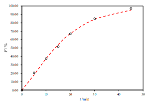
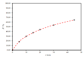
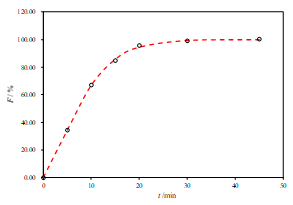
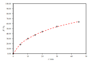
The results from experimental dissolution studies expressed as a percentage of released API vs. time and descriptive analyses for reference and test medicinal products are given in Table 1. The in vitro dissolution profiles of the tablets are shown in Figure 1. Each data point represents a mean of twelve measurements for each sample. In this work, dissolution profiles are compared by different methods belonging to one of three main classes: univariate model-independent, multivariate model-independent, and model-dependent methods.
|
Table 1. In vitro dissolution profiles of reference (R) and test (T) medicinal products
|
||||||||||||||||||||||||||||||||||||||||||||||||||||||||||||||||||||||||||||||||||||||||||||||||||||||||||||||||||||||||||||||||||||||||||||||||||||||||||
|
(a) In vitro dissolution profiles in medium pH 6.8
(b) In vitro dissolution profiles in medium pH 4.5
(c) In vitro dissolution profiles in medium pH 1.2 (HCl, NaCl)
|
||||||||||||||||||||||||||||||||||||||||||||||||||||||||||||||||||||||||||||||||||||||||||||||||||||||||||||||||||||||||||||||||||||||||||||||||||||||||||
Figure 1. In vitro dissolution profiles of reference (R) and test (T) medicinal products
Univariate model-independent approaches
The f1 (difference factor) is proportional to the average difference between the two profiles, whereas f2 (similarity factor) is inversely proportional to the average squared difference between the two profiles. Generally, f1 values up to 15 (0–15) and f2 values greater than 50 (50–100) ensure the similarity of the two curves. The values of f1 and f2 factors for test vs. reference samples are calculated from the means of percent dissolved at each time point (Table 1) by using Eqs. (1) and (2) and listed in Table 2 for all dissolution media.
Table 2. The values of f1 and f2 parameters computed from the experimental dissolution data for reference (R) and test (T) medicinal products
Table 2a. The values of f1 and f2 parameters computed from the experimental dissolution data for reference (R-SL) and test (T) medicinal products at pH 6.8, 4.5 and 1.2
|
Pairwise factors f1 and f2 |
Standard error |
Similarity |
|
|
Phosphate buffer pH of 6.8 |
|||
|
< f1>* |
4.99 |
0.76 |
YES |
|
f1** |
2.00 |
- |
YES |
|
< f2>* |
66.57 |
2.50 |
YES |
|
f2** |
84.12 |
- |
YES |
|
Acetate buffer pH of 4.5 |
|||
|
< f1>* |
11.93 |
1.25 |
YES |
|
f1** |
11.92 |
- |
YES |
|
< f2>* |
59.28 |
2.97 |
YES |
|
f2** |
58.10 |
- |
YES |
|
Buffer pH 1.2 (HCl, NaCl) |
|||
|
< f1>* |
7.06 |
0.50 |
YES |
|
f1** |
6.47 |
- |
YES |
|
< f2>* |
72.63 |
1.36 |
YES |
|
f2** |
75.04 |
- |
YES |
*computed from individual test versus average reference data
**computed from average test versus average reference data
Table 2b. The values of f1 and f2 parameters computed from the experimental dissolution data for reference (R-DE) and test (T) medicinal products at pH 6.8, 4.5 and 1.2
|
Pairwise factors f1 and f2 |
Standard error |
Similarity |
|
|
Phosphate buffer pH of 6.8 |
|||
|
< f1>* |
11.64 |
1.16 |
YES |
|
f1** |
11.55 |
- |
YES |
|
|
|
|
|
|
< f2>* |
44.97 |
3.03 |
NO |
|
f2** |
43.38 |
- |
NO |
|
Acetate buffer pH of 4.5 |
|||
|
< f1>* |
11.58 |
1.24 |
YES |
|
f1** |
11.54 |
- |
YES |
|
|
|
|
|
|
< f2>* |
58.20 |
2.81 |
YES |
|
f2** |
57.22 |
- |
YES |
|
Buffer pH 1.2 (HCl, NaCl) |
|||
|
< f1>* |
7.50 |
0.46 |
YES |
|
f1** |
6.68 |
- |
YES |
|
|
|
|
|
|
< f2>* |
71.08 |
1.30 |
YES |
|
f2** |
73.11 |
- |
YES |
*computed from individual test versus average reference data
**computed from average test versus average reference data
However, in the analyzed data sets, two prerequisites that are essential for the similarity factor f2 to be used as a valid indicator of similarity are not fulfilled, as elaborated before. Results given in Table 1 show that the Relative Standard Deviation (coefficient of variation) is larger than 10 % at several time points in the case of both medicinal products. Calculated f1 and f2 values (Table 2) from dissolution profiles of test vs. reference samples ensured pharmaceutical equivalence with exception of phosphate buffer pH 6.8 where the similarity factor f2 is less than 50 compared to the reference samples from German market. The T/R-DE dissolution profiles gave a non-conclusive result. Using f2 value (44.97) these two dissolution profiles should be considered not similar. But this value is very close to the limit value of 50 and it might be affected with analytical or sampling errors leading to the wrong conclusion about similarity (Type II error; profiles are considered as different when they are similar).
Nevertheless, the f2 values in this context are presented only for comparison purposes and are not applied for making definitive conclusions concerning the similarity of dissolution profiles.
Although the fit factors are easy to calculate, they lack more detailed information about the actual kinetics of the release of API from tablets. At the same time, these parameters do not reflect nor account for the variability (expressed e.g. through the dispersion) associated with each dissolution profile. The f2 is insensitive to the shape of the dissolution profiles and does not take into account the information of unequal spacing between sampling time points. Also, fit factors are simple statistics that cannot be used to exactly (and mathematically rigorously) formulate a statistical hypothesis for assessment of dissolution similarity.
Aside from the analyses based on f1 and f2 parameters (factors), another mathematical comparison with the model-independent method is performed by applying Ratio test procedures comparing the percent of dissolved test/ratio samples (PD), area under the concentration curve (AUC) as well as the average dissolution time (ADT) (Table 3).
Table 3. Ratio test approaches comparing test (T) / reference (R) medicinal product
Table 3a. The ratio of percent dissolved (PD)
|
Ratio <PD> pH 6.8 |
||||||
|
t/min |
5 |
10 |
15 |
20 |
30 |
45 |
|
T/R1(SL) |
1.123 |
0.987 |
1.017 |
1.014 |
1.020 |
0.997 |
|
T/R2(DE) |
0.830 |
0.830 |
0.830 |
0.830 |
0.830 |
0.830 |
|
Ratio <PD> pH 4.5 |
||||||
|
T/R1(SL) |
1.175 |
1.175 |
1.175 |
1.175 |
1.175 |
1.175 |
|
T/R2(DE) |
1.149 |
1.149 |
1.149 |
1.149 |
1.149 |
1.149 |
|
Ratio <PD> pH 1.2 |
||||||
|
T/R1(SL) |
1.048 |
1.048 |
1.048 |
1.048 |
1.048 |
1.048 |
|
T/R2(DE) |
1.121 |
1.121 |
1.121 |
1.121 |
1.121 |
1.121 |
Table 3b. The ratio of area under the concentration curve (AUC)
|
Ratio <AUC> pH 6.8 |
||||||
|
t/min |
5 |
10 |
15 |
20 |
30 |
45 |
|
T/R1(SL) |
1.123 |
1.057 |
1.029 |
1.023 |
1.020 |
1.015 |
|
T/R2(DE) |
0.830 |
0.800 |
0.791 |
0.804 |
0.855 |
0.909 |
|
Ratio <AUC> pH 4.5 |
||||||
|
T/R1(SL) |
1.149 |
1.158 |
1.164 |
1.163 |
1.151 |
1.113 |
|
T/R2(DE) |
0.830 |
0.800 |
0.791 |
0.804 |
0.855 |
0.909 |
|
Ratio <AUC> pH 1.2 |
||||||
|
T/R1(SL) |
1.124 |
1.110 |
1.085 |
1.046 |
0.990 |
0.965 |
|
T/R2(DE) |
1.121 |
1.104 |
1.090 |
1.067 |
1.010 |
0.969 |
Table 3c. Ratio of average dissolution time (ADT)
|
Ratio <ADT> pH 6.8 |
||||||
|
t/min |
5 |
10 |
15 |
20 |
30 |
45 |
|
T/R1(SL) |
1.000 |
0.922 |
0.984 |
0.986 |
0.998 |
0.953 |
|
T/R2(DE) |
1.000 |
0.949 |
1.002 |
1.081 |
1.319 |
1.350 |
|
Ratio < ADT > pH 4.5 |
||||||
|
T/R1(SL) |
1.000 |
0.970 |
1.012 |
1.024 |
0.980 |
0.918 |
|
T/R2(DE) |
1.000 |
1.013 |
1.011 |
0.987 |
0.979 |
0.886 |
|
Ratio < ADT > pH 1.2 |
||||||
|
T/R1(SL) |
1.000 |
0.975 |
0.897 |
0.867 |
0.928 |
0.975 |
|
T/R2(DE) |
1.000 |
0.970 |
0.975 |
0.897 |
0.867 |
0.971 |
From the obtained results for PD, AUC, and ADT ratios in all dissolution media for the compared test and reference medicinal product (purchased form Slovenian market) were within the limits that are usually considered acceptable to establish the similarity between dissolution profiles.
Moreover, the values obtained for the calculated ADT ratios in the medium pH 6.8 between the test and the reference medicinal product from the German market was not within the 90% confidence interval for a sampling time of 30 and 45 minutes.
These model-independent procedures reflect only the major or minor similarities between these two profiles and can be considered as a good tool to judge its dissolution equivalence. However, the acceptance criteria here are also more or less doubtful.
In the FDA guideline for industry, the procedure allows the use of mean data and recommends that the Relative Standard Deviation (RSD) at an earlier time point (for example 5 or 10 minutes) not be more than 20%, and at other time points not more than 10%.
Therefore, to provide a more accurate, statistically justified conclusion, analysis based on the model-independent method based on generalized statistical distance and model-dependent method, coupled with a multivariate statistical approach was accomplished.
For the present study, the multivariate statistical analysis using both the non-transformed data for the fitting parameters, as well as the natural logarithm (ln) transformed data is performed. This was done to clarify the possible ambiguity in the assumption for the multivariate normal distribution of the model parameters, which has been discussed to some extent in the literature [13, 14]. However, in the presently studied case, conclusive results both with transformed and non-transformed model parameters are obtained.
Multivariate model-independent approach based on generalized statistical distance
In a case of intra-batch (within-batch) variability, it is generally recommended that multivariate statistical methods be judged on the in vitro similarity between the dissolution profiles of the test and the reference medicinal product. A multivariate method, known as Hotelling’s T2 test, can also be used to test the coincidence hypothesis described earlier. Tsong et al. describe a multivariate method that uses the Mahalanobis distance, which takes the variability and correlation structure into account in measuring the difference between mean dissolution profiles. The methods based on the mixed-effects model and the multivariate Hotelling’s T2 method are not mentioned in any FDA оr ЕМА guidance documents. This method can be thought of as a multivariate analog of the two one-sided t-test procedures used in the assessment of average bioequivalence. The multivariate confidence region has often been used to describe the variation of estimation of DM. The decisions of similarity can be made with an appropriate comparison of the confidence limits of the estimated metric with a prespecified similarity limit ∆DM. The 90% confidence limits of DM can be obtained from the multivariate confidence region of the expected values of xtest and xref (the sample means), under the multivariate normal assumption. The results based on Mahalanobis distance computed between the test formulations and the two reference formulations are presented in Table 4.
Table 4. Mahalanobis distance between reference (R) and test (T) medicinal products
|
F(d,pT + pR-d-1, 090)=2.1524 K=0.7727 |
DM |
90% Cl-low |
90% Cl-high |
DM lim. |
Similarity |
|
pH 6.8 |
|
|
|
|
|
|
T/R1(SL) |
2.9033 |
1.2344 |
4.5723 |
11.1964 |
YES |
|
T/R2(DE) |
2.3389 |
0.6699 |
4.0078 |
13.8514 |
|
|
pH 4.5 |
|||||
|
T/R1(SL) |
2.6078 |
0.9388 |
4.2768 |
10.2576 |
YES |
|
T/R2(DE) |
3.3750 |
1.7061 |
5.0440 |
10.5292 |
|
|
pH 1.2 |
|||||
|
T/R1(SL) |
2.0350 |
0.3361 |
3.7040 |
9.4479 |
YES |
|
T/R2(DE) |
1.6675 |
-0.0015 |
3.3364 |
10.9689 |
|
When looking at the results from the performed multivariate method, it is obvious that these dissolution profiles can be considered as similar.
Multivariate model-dependent approach
Mathematical models have been used extensively for the parametric representation of dissolution data. After fitting several models to the individual unit dissolution data, the selection was based on the comparisons of the following features of the models: (1) higher determination coefficient, (2) smaller absolute difference between each fitted and actual percent dissolved, and (3) smaller residual mean square. Considering these criteria, the Weibull model function was that which fit best to the dissolution data of reference and test products. Weibull distribution is often able to describe S-shaped, sigmoidal dissolution profiles.
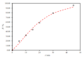
According to the β (shape factor), parameters of test product was found not to be different from those of reference product, implying that the dissolution profiles of the test product were similar to the profile of both reference products (Figure 2 and 3).
a.
b.
c.
Figure 2. Representative fits of two sets of data for the R1-SL with two-parameter Weibull model function (a. pH 6.8, b. pH 4.5 and c. pH 1.2)
Table 5. Two-parameter Weibull model function – logarithmic (ln) transformation of data for fitting parameters between reference (R) and test (T) medicinal products
|
F(d,pT + pR-d-1, 090)=2.5746 K=2.8636 |
DM |
90% Cl-low |
90% Cl-high |
DM lim. |
Similarity |
|
pH 6.8 |
|
|
|
|
|
|
T/R1(SL) |
0.3044 |
-0.6437 |
1.2526 |
2.4420 |
YES |
|
T/R2(DE) |
2.4671 |
1.5189 |
3.4152 |
3.6959 |
|
|
pH 4.5 |
|||||
|
T/R1(SL) |
1.5982 |
0.6501 |
2.5464 |
3.5903 |
YES |
|
T/R2(DE) |
2.1732 |
1.2250 |
3.1214 |
4.6178 |
|
|
pH 1.2 |
|||||
|
T/R1(SL) |
1.2918 |
0.3436 |
2.2400 |
9.0216 |
YES |
|
T/R2(DE) |
1.4844 |
0.5362 |
2.4326 |
5.4002 |
|
a.
b.
c.
Figure 3. Representative fits of two sets of data for the R2-DE with two-parameter Weibull model function (a. pH 6.8, b. pH 4.5 and c. pH 1.2)
The shape parameter, β, characterizes the profile as either exponential (β =1), S-shaped with upward curvature followed by a turning point (β >1), or as one with steeper initial slope than consistent with the parabolic (β <1). β –Values greater than 1 for test products were similar to those of the reference products indicating that their overall dissolution profiles are similar. Among the four models, Weibull was an excellent model and possessed parameters that were sensitive to the ranges of dissolution profiles.
The accomplishment of the dissolution similarity profile was supportive data in the development of test formulation as well as in the establishment of in vitro/in vivo correlation.
Conclusion
The objectives of this work were to apply many profile comparison approaches to dissolution data to show in vitro similarity between developed test formulation and two reference products from different markets. Three general approaches to compare dissolution profiles were examined; they are independent-model procedures, such as difference (f1) and similarity (f2) factors; Ratio test methodology; a multivariate model-independent approach based on generalized statistical distance (Mahalanobis distance) and the model-dependent approach based on the Weibull model function used to fit the dissolution profiles. Nevertheless, fit factors appear to be inapplicable and of little use in comparing dissolution profiles, because one of the regulatory requirements was not achieved. Therefore, a multivariate model-independent method based on Mahalanobis generalized statistical distance was used which takes the variability and correlation structure into account in measuring the difference between mean dissolution profiles. Hence, according to the obtained data the dissolution profile can be considered as similar.
Furthermore, a model-dependent approach (based on the utilization of the Weibull model function), sequentially followed by the analysis of the fitting parameters based on generalized statistical distance has shown the best performance, with model parameters sensitive to the tested range of dissolution profiles. This approach provides extra arguments in making the decision about the actual significant similarity between the test and the references medicinal product, allowing a better description of the dissolution process and thus a better prediction of in vivo performance, which is the ultimate goal in comparing potential therapeutically equivalent products.
The obtained results from the comparative dissolution analysis indicated a definitive conclusion on a similarity of the in vitro dissolution profiles between the Metformine film-coated tablets and the two references medicinal product from different markets. Implemented statistical methods can be considered as a regulatory accepted concept for evaluation of in vitro similarity of generic medicines.
Conflict of interests: The authors declare no conflicts of interest.
References